
Plumes of carbon dioxide in the simulation swirl and shift as winds disperse the greenhouse gas away from its sources. The simulation also illustrates differences in carbon dioxide levels in the northern and southern hemispheres and distinct swings in global carbon dioxide concentrations as the growth cycle of plants and trees changes with the seasons.
The carbon dioxide visualization was produced by a computer model called GEOS-5, created by scientists at NASA Goddard Space Flight Center’s Global Modeling and Assimilation Office.
The visualization is a product of a simulation called a “Nature Run.” The Nature Run ingests real data on atmospheric conditions and the emission of greenhouse gases and both natural and man-made particulates. The model is then left to run on its own and simulate the natural behavior of the Earth’s atmosphere. This Nature Run simulates January 2006 through December 2006.
While Goddard scientists worked with a “beta” version of the Nature Run internally for several years, they released this updated, improved version to the scientific community for the first time in the fall of 2014.
The visualization was created using output from the GEOS modeling system, developed and maintained by scientists at NASA. The height of Earth’s atmosphere and topography have been vertically exaggerated and appear approximately 400 times higher than normal to show the complexity of the atmospheric flow.
Measurements of carbon dioxide from NASA’s second Orbiting Carbon Observatory (OCO-2) spacecraft are incorporated into the model every 6 hours to update, or “correct,” the model results, called data assimilation.
As the visualization shows, carbon dioxide in the atmosphere can be mixed and transported by winds in the blink of an eye. For several decades, scientists have measured carbon dioxide at remote surface locations and occasionally from aircraft. The OCO-2 mission represents an important advance in the ability to observe atmospheric carbon dioxide. OCO-2 collects high-precision, total column measurements of carbon dioxide (from the sensor to Earth’s surface) during daylight conditions.
While surface, aircraft, and satellite observations all provide valuable information about carbon dioxide, these measurements do not tell us the amount of carbon dioxide at specific heights throughout the atmosphere or how it is moving across countries and continents.
Numerical modeling and data assimilation capabilities allow scientists to combine different types of measurements (e.g., carbon dioxide and wind measurements) from various sources (e.g., satellites, aircraft, and ground-based observation sites) to study how carbon dioxide behaves in the atmosphere and how mountains and weather patterns influence the flow of atmospheric carbon dioxide.
Scientists can also use model results to understand and predict where carbon dioxide is being emitted and removed from the atmosphere and how much is from natural processes and human activities.
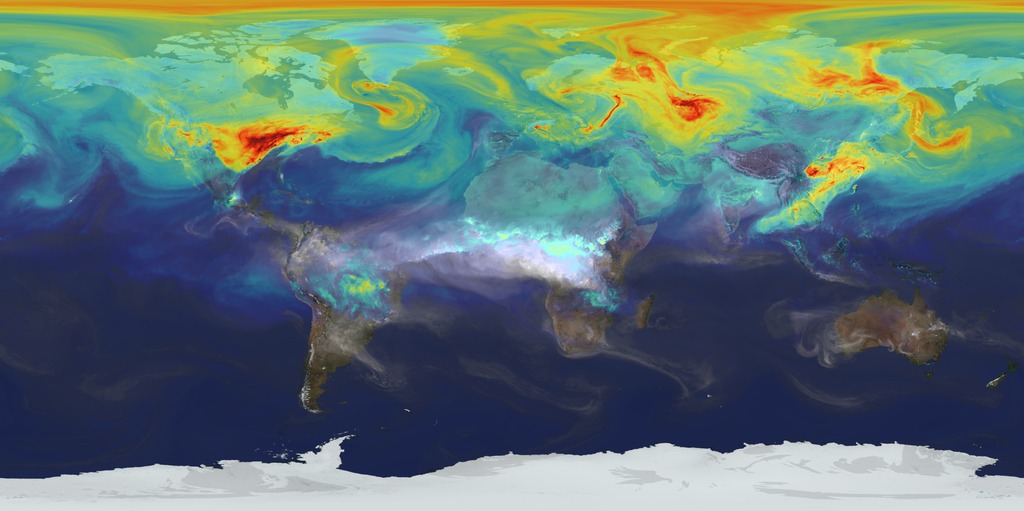
Carbon dioxide variations are largely controlled by fossil fuel emissions and seasonal fluxes of carbon between the atmosphere and land biosphere. For example, dark red and orange shades represent regions where carbon dioxide concentrations are enhanced by carbon sources.
During Northern Hemisphere fall and winter, when trees and plants begin to lose their leaves and decay, carbon dioxide is released in the atmosphere, mixing with emissions from human sources. This, combined with fewer trees and plants removing carbon dioxide from the atmosphere, allows concentrations to climb all winter, reaching a peak by early spring.
During Northern Hemisphere spring and summer months, plants absorb a substantial amount of carbon dioxide through photosynthesis, thus removing it from the atmosphere and change the color to blue (low carbon dioxide concentrations). This three-dimensional view also shows the impact of fires in South America and Africa, which occur with a regular seasonal cycle.
Carbon dioxide from fires can be transported over large distances, but the path is strongly influenced by large mountain ranges like the Andes. Near the top of the atmosphere, the blue color indicates air that last touched the Earth more than a year before. In this part of the atmosphere, called the stratosphere, carbon dioxide concentrations are lower because they haven’t been influenced by recent increases in emissions.
Scientists are using climate models like this one — called GEOS-5 (Goddard Earth Observing Model, Version 5, created at NASA’s Goddard Space Flight Center) — to better understand how carbon dioxide moves around Earth’s atmosphere and how carbon moves through Earth’s air, land and ocean over time. Rising carbon dioxide levels in the atmosphere are driving Earth’s ongoing climate change.
This animation shows a five-day period in June 2006. The model is based on real emissions inventory data and is then set to run so that scientists can observe how the greenhouse gas behaves in the atmosphere once it has been emitted.
